Hypothesis Test Sample Size and Power

These all start from the moment when I saw the post: http://datapirates.blogspot.de/2016/03/why-ab-testing-sucks.html. It claims A/B test, which is exactly two sample t-test, is useless. Below is the simulation running with R.

Let’s do some experiments!

First, we generate two random vectors a and b. In this case, the average of a is 0.1467 while the average of b is 0.19. Both vector a and b are made by binary element, and the ideal average of a is 0.15, while the average of b is 0.2.

#init
sample_s <-300
b_threshold <- 20
a_threshold <- 15
set.seed(106)
a <- (sample(x = 100,size = sample_s,replace=T)<a_threshold)*1
b <- (sample(x = 100,size = sample_s,replace=T)<b_threshold)*1

Next, let’s do a simple two sample t-test.

test <- t.test(b, a, alternative = "greater")
t <- test$statistic
degree <- test$parameter
sigma <- sd(b - a)
ncp <- (b_threshold - a_threshold)/100 * sqrt(sample_s/2)/sigma
cat("p.value:", test$p.value, "power:", 1 - pt(q = t, df = degree, ncp = ncp))

## p.value: 0.07829374 power: 0.3954021

Here we got p-value = 0.07, if we set type I error threshold to 0.05, we can not reject the Null hypothesis. However, does that means we should accept Null hypothesis and believe mean of vector a and b are same? No!. Maybe it is easy to understand this way: if we accept null hypothesis and believe there is no difference between a and b, we have 61% to make a mistake (type II), while if we reject Null hypothesis now, we have ~7% to make mistake (type I). The reason why we control type I error is that we can’t take the risk making that mistake. In another word, if we only have 300 samples each group and want to see if conversion rate improve or not, the answer should be NO.

Next, let’s calculate the possible maximum power given alpha, sample size, alternative (or effect size?) under the normal assumption. Below are the power and Null/alternative distribution. We can see that power reach 80% when we have more than 690 samples (in each group), and it is obvious 300 samples is not enough. Also, we can see that actually when we have 300 samples in each group, the distribution charts are close. Frankly speaking, two sample mean hypothesis test is nothing but compare mean of two samples, taking variance, central limit theorem into consideration and use distribution to measure the probability.

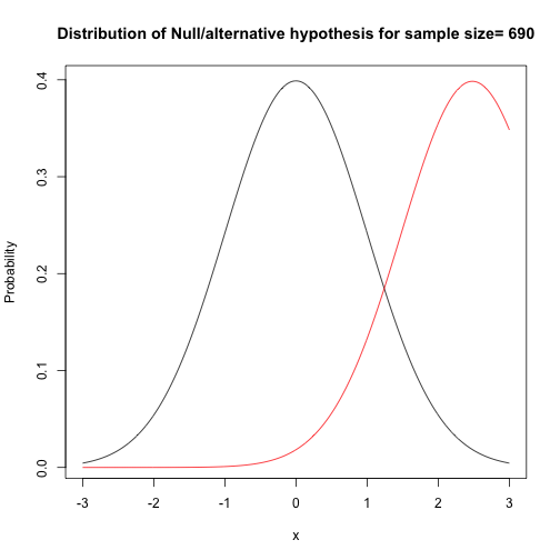
## power: 0.7984382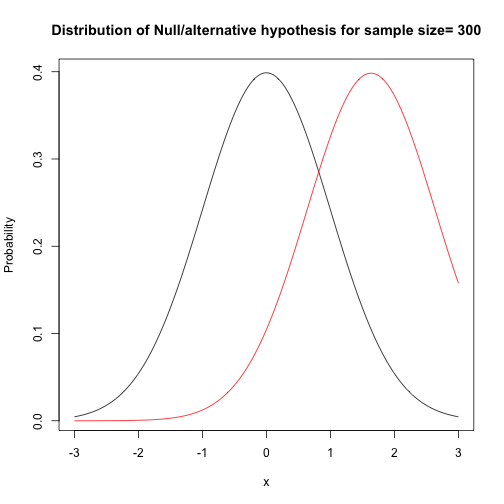

## power: 0.4959953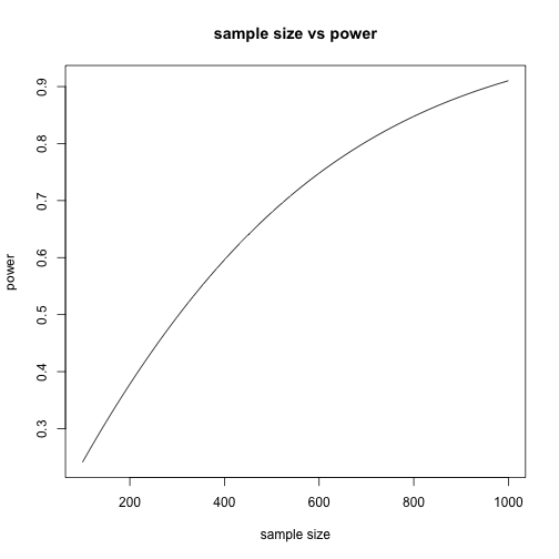

Actually, what the author in that post is doing, is similar to calculating the power of the test. Since the power of the test is that: under the assumption that alternative hypothesis is correct, the probability of rejecting the Null hypothesis. He runs 100 simulations and found out ~50% reject and ~50% accept, which is near the power 0.57 that we are seeing in the above graph.

R has built in function to calculate sample size given type I error(alpha), type II error(beta), expected mean difference (delta), and data standard deviation. I also include calculation by hand under the normal assumption.

#calculate sample size

alpha <- 0.05
beta <- 0.2
delta <- 0.05
pool.sd <- sqrt((var(a)+var(b)))
c1 <- qnorm(p = 1-alpha,mean = 0,sd = 1)
c2 <- qnorm(p = 1-beta,mean = 0,sd = 1)
(ideal.sample.norm <- (c1+c2)^2/(delta/pool.sd)^2)

## [1] 692.4188

power.t.test(delta=delta,sd=sqrt(pool.sd^2/2),sig.level=alpha,power=1-beta,type="two.sample",alternative="one.sided")

## 
##      Two-sample t test power calculation 
## 
##               n = 693.0962
##           delta = 0.05
##              sd = 0.3741583
##       sig.level = 0.05
##           power = 0.8
##     alternative = one.sided
## 
## NOTE: n is number in *each* group

The first method is based on normal distribution. But there is a little flaw here since I use “sample pool variance” to replace variance under assumption distribution, and mean variance is the function of sample size. It is interesting that I found in power.t.test function, the sd is standard deviation in each group, not mean-variance or total variance… (Actually I just followed the formula I found online above).

After trying to derive sample estimation formula by myself, I have the following result:

##two sample z test (binomial) model

alpha <- 0.05
beta <- 0.2
p1 <- 0.15;p2 <- 0.2;delta <- abs(p1-p2)
p.sd <- sqrt(p1*(1-p1)+p2*(1-p2))
c1 <- qnorm(p = 1-alpha,mean = 0,sd = 1)
c2 <- qnorm(p = beta,mean = 0,sd = 1)
(ideal.sample.norm2 <- (p.sd*(c1-c2)/delta)^2)

## [1] 710.9941

#use build in function

power.prop.test(power=.8,p1=.15,p2=.2,sig.level=0.05,alternative = "one.sided")

## 
##      Two-sample comparison of proportions power calculation 
## 
##               n = 713.0383
##              p1 = 0.15
##              p2 = 0.2
##       sig.level = 0.05
##           power = 0.8
##     alternative = one.sided
## 
## NOTE: n is number in *each* group

This result looks reasonable.

Conclusion

Statistical A/B test or hypothesis test, is a very good technique to solve the real world problem. However, understanding more about underlying assumption and requirement is important in real world. In practical use cases, we don’t need to be 100% analytical precise (like use sample variance to conduct lazy calculation won’t change result a lot), but we do need to understand the problem and the techniques that we are trying to use.